|
NSCL DDAS
1.0
Support for XIA DDAS at the NSCL
|
|
NSCL DDAS
1.0
Support for XIA DDAS at the NSCL
|
Sometimes an experiment being read out by the NSCL Digital Data Acquisition System (DDAS) will require more than one crate. You might find yourself in this situation if your experiment has more channels to read out than are possible to fit into a single crate. Regardless of the reason, setting up a multi-crate system is similar in many respects to setting up a single crate system. There are however a few extra steps that are important to get right for the system to operate correctly. In this document, the reader will learn:
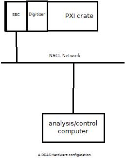
DDAS data acquisition and online analysis rely on several hardware and software components.
The figure below shows a simple DDAS hardware configuration:
The figure below shows a simple DDAS software configuration emphasizing the data flow.
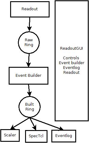
A few points are worth noting:
Finally a bit about where the DDAS support software is installed at the NSCL. The NSCL may have several versions of the DDAS software installed concurrently. In general these will be installed in
/usr/opt/ddas/version
Where version above is a software version number of the form major.minor-editlevel major, minor and editlevel are three numbers that are called the major version the minor version and the edit level. Edit level changes reflect defect fixes and very small enhancements. minor version changes reflect enhancements and fixes that are somewhat more involved. Migrating to versions where only the minor version changed will at most require you to recompile without any need to modify your code. Major version changes are very significant fixes and enhancements that may require changes being made to any user-level code.
In addition to these there is a symbolic link /usr/opt/ddas/current that points to the version of the DDAS software that is recommended for use. This link will only change during significant accelerator shutdowns.
Each version's top-level directory includes a script ddassetup.bash
Source that script into your interpreter to setup several environment variables:
DDAS_ROOT - points to the top level ddas installation directory (that's the directory that holds the ddassetup.bash script).DDAS_BIN - points to $DDAS_ROOT/bin this directory contains all executable programs.DDAS_LIB - points to the $DDAS_ROOT/lib directory. This contains all of the link libraries DDAS applications might need to link against.DDAS_INC - points to $DDAS_ROOT/include a directory that contains all header files DDAS applicatons may need.DDAS_SHARE - points to $DDAS_ROOT/share this directory tree contains documentation, program skeletons and scripts.The remainder of this document will assume that you have selected a DDAS version and sourced its ddassetup.bash script into your shell.
Many of the DDAS software components require a set of configurations files to be in the current working directory. These configuration files describe the configuration of modules in a crate and point at a settings file containing the parameters used by the digital pulse processing (DPP) algorithms for each module in use.
These files are described in the documentation of readout . This section will summarize the files needed for nscope. By convention, a directory tree is used to hold the configuration files for each crate. The tree looks like this:
home-directory
     |
     +-- readout
            |
            +--- crate_1  (configuration for crate 1).
            +--- crate_2  (configuration for crate 2).
            ...
            +--- crate_n  (configuration for last crate, n).
Since we have two crates, this should look like:
Home directory
   |
   +---readout
          |
          +--- crate_1
          |      +--- cfgPixie16.txt
          |      +--- pxisys.ini
          |      +--- crate_1.set
          |      +--- modevtlen.txt
          +--- crate_2
                 +--- cfgPixie16.txt
                 +--- pxisys.ini
                 +--- crate_2.set
                 +--- modevtlen.txt
The directory $DDAS_SHARE/readout/crate_1 has sample configuration files that can be copied into your experiment account so you don't need to start from scratch.
cfgPixie16.txt - Indicates which modules are in which crates.pxisys.ini - Describes the PCI layout of the crate for the XIA API.crate_1.set - A parameter settings file.modevtlen.txt - Describes the number of 32-bit words in an event for each module.Once you've created ~/readout/crate_1 and ~/readout/crate_2, finish making the structure below by
cp $DAQ_SHARE/readout/crate_1/* ~/readout/crate_1
cp $DAQ_SHARE/readout/crate_2/* ~/readout/crate_2
mv ~/readout/crate_2/crate_1.set ~/readout/crate_2/crate_2.set
Then modify the last line of ~/readout/crate_2/cfgPixie16.txt to contain the path ~/readout/crate_2/crate_2.set.
Of these files:
pxisys.ini must not be modified unless you are using a non-standard crate.cfgPixie16.txt must be modified to reflect the layout of modules in your crate and the actual desired name of the parameter settings file. The format of the cfgPixie16.txt file is described in detail at The cfgPixie16.txt format. nscope and Readout both use this file.crate_1.set should be renamed to match the final settings file path name in .txt This settings file contains the DPP parameters nscope and Readout load into the digitizers and is written by nscope if desired.modevtlen.txt must be modified to reflect the actual event sizes selected for each module. This must be modified to reflect the number of modules in cfgPixie16.txt and the sizes must be modified appropriately if waveforms are being acquired.At the NSCL, all spdaqs mount a network file system which makes your crate_1 and crate_2 directories accessible on all systems automatically. Just because the directories are there in the file system, doesn't mean that the hardware is attached to the system. In fact, the only thing that will differentiate what settings file you use is which directory you are in when you launch any of the DDAS programs. This will be important later on.
Communication with the Pixie-16 modules requires communication over the PXI backplane. In any of the DDAS systems at the NSCL, whether using a fiber interface of embedded single board computer (SBC), a PLX 9054 chip is involved in this communication. There is a kernel module that must be loaded into the kernel prior to using this chip. You can load it by :
sudo /usr/opt/plx/Bin/Plx_load 9054
You will be asked to enter you password and then on success you will get the following output written to the terminal
Install: Plx9054
  Load module......... Ok (Plx9054.ko)
  Verify load......... Ok
  Get major number.... Ok (MajorID = 251)
  Create node path.... Ok (/dev/plx)
  Create nodes........ Ok (/dev/plx/Plx9054)
The user must load the PLX kernel module before using DDAS after every time the computer is booted.
The DDAS is based on the XIA Pixie-16 digitizer. There are three flavors of these hardware in use at the NSCL and they vary based on the ADC sampling rate and resolution. You can read more about them at The Pixie Digitizers. In the following sections, we will assume that we are using the 100 MSPS modules with 12-bit resolution. The other aspect of this that needs some addressing is the
The digitizers need to be modified to properly distribute a clock and triggers in a multicrate system. This is done by changing jumper settings on the digitizers and connecting up a trigger distribution board.
Each module has a jumper block, JP101, on the board that must be configured according to its role in the multi-crate system. There are three classes of modules in a multicrate system and the jumper settings must be adjusted to reflect these. The classes are
| Class | Abbrev | Description |
|---|---|---|
| Multi-crate clock master | MCCM | The multi-crate master is the source of the clock that will be distributed to all other Pixie-16s in the system. There is only one of these. The multi-crate master resides in slot 2 of the master crate. |
| Crate clock master | CCM | There are as many crate masters as there are crates in the system. It receives the clock from the MCCM and distributes it to the other modules in its crate. Note that the MCCM is the crate master of its crate. Crate masters reside in slot 2. |
| Clock recipient | CR | All modules that are neither an MCCM or CCM are clock recipients. |
To sum up, each crate will have a clock master and in one of those crates, the clock master will be the multi-crate clock master. All other modules in the system will be recipients of the clock. Keep in mind that all Pixie-16 modules are the same and can serve any of these roles, so you need not stress making the decision of which module is to serve which role. Modules that are in slot 2 are the CCMs and one of those will be the MCCM.
The next step is to configure the jumpers for each module in the system according to the role that the module will serve. The jumper settings are extremely important to get right because if the modules are configured incorrectly, the host computer that is reading out the hardware can completely lock up. You would then have to reboot the crate and the computer.
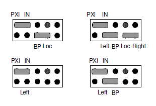
In the crate that we will consider the master crate, we will set the jumpers of the module in slot 2 to look like the configuration in the top right of the diagram above. All other modules in that master crate are clock recipients and should have their jumpers configured like the configuration shown in the bottom left. For all other crates in the system, the module in slot 2 should have its jumpers configured as in the bottom right. These are the crate clock masters. All remaining modules in the system are clock recipients and will have their jumpers configured as in the bottom left of the above diagrams.
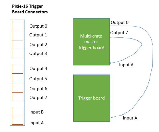
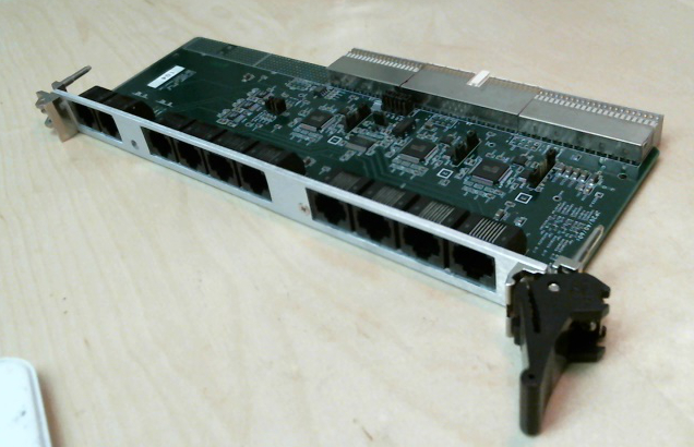
In order to send the clock between the crates, a Pixie-16 trigger distribution board must be plugged into the rear of each chassis in the system. The Pixie-16 Trigger Board should be plugged into the rightmost slot in the rear of the crate so that it is immediately behind the module in slot 2. The trigger board is an essential piece of hardware used to connect the system together. It distributes the clock from the multicrate master module and passes it to the crate masters in each of the crates. Those crate masters then are responsible for distributing it to the other modules in they system by putting it on the backplane. To connect the system up, the user must connect these boards together.
There are three groups of connectors on the trigger board. The bottom group consists of two connectors and these are inputs A and B. The topmost group consists of four connectors and these are outputs 0 - 3, in order from top to bottom. The middle of group of connectors are outputs 4-7, once again in order from top to bottom. Each crate in the system must have one of these installed in the rear of the crate, immediately behind the slot 2 position on the front where the crate master resides. The trigger board in the master crate (immediately behind the multicrate master module), will need to connect one of the outputs to its own input A. A second output should then be connected to input A of the other crate. This wiring scheme looks like this:
The cables that are used to connect the trigger boards should be at least CAT5 cable.
The trigger board is configured with jumpers. At the NSCL, we don't typically stray from a standard configuration. Make sure that the following pins are set for the jumpers on all of your trigger boards:
| Jumper | Default Connections |
|---|---|
| JP20 | 2-3, 6-7 |
| JP40 | 2-3, 6-7 |
| JP60 | 1-2, 7-8 |
| JP21 | normal |
| JP41 | normal |
| JP61 | reverse |
| JP1 | P16 |
| JP100 | Connect to J4 |
| JP101 | Connect to J4 |
| JP102 | Connect to J4 |
| JP103 | Connect to J4 |
| JP104 | Connect to J4 |
| JP105 | Connect to J4 |
With the clock jumpers in the correct configuration, it is essential that we wire up the rest of the system. For each crate, it is necessary that you have a corresponding data collection computer attached to the crate. You can either accomplish this with a fiber interface or an embedded single board computer in slot 1 of each crate. To read out the crate with a fiber interface, a fiber interface card must be installed in slot 1 and then the data collection computer must have a compatible PCI bridge card installed. These of course must be connected via a fiber optic cable.
The next step to get the system running is to configure each module for taking data. As was already discussed in the Single-crate System Setup Tutorial section, the parameters controlling pulse processing are programmable via software. The DDAS provides the nscope application to address this issue. There are an abundance of parameters that are able to be controlled with nscope and not all configurations are sensible. In this section, I will describe the basic approach to configure a single channel for data taking and then will describe some specific settings that need to be enabled for multi-crate operation.
The nscope application must be told basic information about the system it is intended to configure at start up. It receives this information through the cfgPixie16.txt file that it expects to exist in the directory it was launched in.
The cfgPixie16.txt is a very simple file that has the following form:
Crate Id (not used)
Number of modules in crate
Slot of 1st module
Slot of 2nd module
...
Slot of Nth module
Path to parameter file (.set)
You will need to modify each one of these that is associated with your crates. For this setup, we have two crates and thus I will have to modify the one in the crate_1 and crate_2 directories. In crate 1, I have two modules present, one in slot 2 and one in slot 3. The corresponding cfgPixie16.txt file will be:
1
2
2
3
/users/0400x/readout/crate_1/crate_1.set
In crate 2, I have three modules in slots 2, 3, and 4. The corresponding cfgPixie16.txt file has the following content:
2
3
2
3
4
/user/0400x/readout/crate_2/crate_2.set
The nscope application will expect to find a cfgPixie16.txt file in the directory it was launched from when it starts up. To launch nscope for configuring crate 1, you therefore need to run:
cd ~/readout/crate_1/.
$DDAS_BIN/nscope
The cfgPixie16.txt file that it reads in will be used to teach it what modules are available in the system to be configured. When you start up nscope, you should see output that looks something like this:
Reading Firmware Version file... DDASFirmwareVersions.txt
Found Firmware    #[FPGAFirmwarefiles]
test: ../firmware/syspixie16_revfgeneral_adc500mhz_rxxxxx.bin
Reading config file... cfgPixie16.txt

2 modules, in slots: 2 3

current working directory /user/0400x/readout/nscope
The textual output that nscope printed should match the information in the cfgPixie16.txt file. If it has conflicting information, then you have probably launched nscope in a different directory than the cfgPixie16.txt you thought you configured.
The very first step is to press "Boot" at this stage. If you have set up the system correctly, this should print a whole lot of output to the terminal and then transition to a state that says the system booted successfully.
Reading Firmware Version file... DDASFirmwareVersions.txt
Found Firmware    #[FPGAFirmwarefiles]
test: ../firmware/syspixie16_revfgeneral_adc500mhz_rxxxxx.bin
Reading config file... cfgPixie16.txt

2 modules, in slots: 2 3

Booting all Pixie-16 modules...

Booting Pixie-16 module #0, Rev=12, S/N=184, Bits=12, MSPS=100
ComFPGAConfigFile:  /user/ddas/ddasDaq/standard/LucidXIA/test100/firmware/syspixie16.bin
SPFPGAConfigFile:   /user/ddas/ddasDaq/standard/LucidXIA/test100/firmware/fippixie16.bin
DSPCodeFile:        /user/ddas/ddasDaq/standard/LucidXIA/test100/dsp/Pixie16DSP.ldr
DSPVarFile:         /user/ddas/ddasDaq/standard/LucidXIA/test100/dsp/Pixie16DSP.var
--------------------------------------------------------

Start to boot Communication FPGA in module 0
Start to boot signal processing FPGA in module 0
Start to boot DSP in module 0

Booting Pixie-16 module #1, Rev=12, S/N=168, Bits=12, MSPS=100
ComFPGAConfigFile:  /user/ddas/ddasDaq/standard/LucidXIA/test100/firmware/syspixie16.bin
SPFPGAConfigFile:   /user/ddas/ddasDaq/standard/LucidXIA/test100/firmware/fippixie16.bin
DSPCodeFile:        /user/ddas/ddasDaq/standard/LucidXIA/test100/dsp/Pixie16DSP.ldr
DSPVarFile:         /user/ddas/ddasDaq/standard/LucidXIA/test100/dsp/Pixie16DSP.var
--------------------------------------------------------

Start to boot Communication FPGA in module 1
Start to boot signal processing FPGA in module 1
Start to boot DSP in module 1
Boot all modules ok
DSPParFile:        /user/0400x/readout/crate_1/crate_1.set
Note that the second to last line states that the modules all booted "ok". That is when you know that the system is ready. You should also see that the status indicator on nscope turns blue and states "System booted".
Now that we have booted our system, we can begin to configure it. This is really a job of repeating the same steps over and over again. Once you learn to configure one channel appropriately, you just repeat the same steps for all other channels in the system.
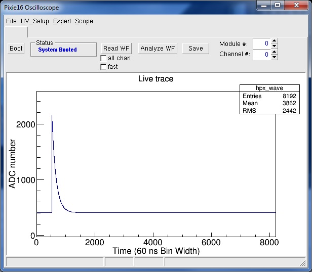
We will begin with the analog signal conditioning parameters. Before the input signal ever reaches the flash ADCs in the digitizers, they are sent through some analog electronics to adapt the signal for digitization. The signal's polarity, baseline offset, and gain can be adjusted in this stage. In order to set the waveform conditioning parameters, you must look at a waveform. Click the Read WF button. If the digitizer does not capture a full waveform, click it again until one is captured.
For the pulser I used, here's a sample picture:
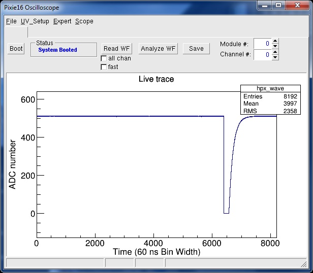
There are two things wrong with this signal:
Click the UV_Setup->Analog Signal Conditioning menu entry. This brings up a screen that looks like this:
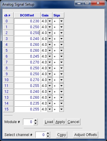
Our pulser is plugged into channel 0 which has the Sign set to + Using the pull down on that channel to set the sign to - (be sure to click Apply to load the setting into the module) and acquiring another trace gives:
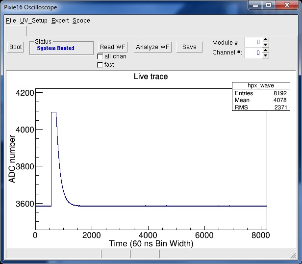
Our trace is still saturating the ADC. We'll next adjust the trace baseline. Do this by clicking the Adjust Offsets button of the Analog Signal Setup control panel.
Reading another waveform then gives:
Our next step is setup the constant fraction (CFD). nscope can compute the parameters it thinks are appropriate. Click the Analyze WF button. The terminal window will output something like:
Filter parameters (From Modules):
    ADC sample deltaT (ns): 60
    Fast rise (ns):         500
    Fast flat (ns):         100
    Energy rise (ns):       6000
    Energy flat (ns):       480
    Tau (ns):               40320
    CFD delay:              80
    CFD scale:              0
Trigger Filter Rise Time is NOT an integer number of dT.  Fixing Now.
Trigger Filter Gap Time is NOT an integer numnber of dT. Fixing Now.
Energy Filter Rise Time is NOT an integer number of dT.  Fixing Now.
CFD Delay is NOT an integer numnber of dT. Fixing Now.
Filter parameters used for ''Analyze Waveform''
Note: Parameters have NOT been altered for the aquisition
    Fast rise (ns):         540
    Fast flat (ns):         120
    Energy rise (ns):       6000
    Energy flat (ns):       480
    CFD delay (ns):         120
Baseline: 410
Since we chose a signal with a good rise and fall time initially, we only care about the computed CFD delay. Click the UV_Setup->CFD to bring up the CFD control panel:
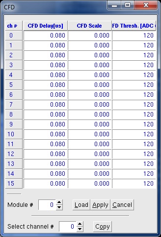
Apply the settings. Finally enable the CFD by selecting UV_Setup->CSRA and setting the CF bit in all of the channels for which you are going to use the CFD. There are numerous options that can be enabled or disabled in the CSRA and CSRB dialogs that are not being discussed here. If you want to know more about the meanings of each bit, you can find information at nscope.
Now that the trigger is set up you can take data and look at the module histograms. Use the menu entry Expert->Start Run this makes the module start taking triggers and histogramming the energy computed from the waveforms. The Read Histo button will read and display the channel energy histogram accumulated by the module. For my pulser I got:
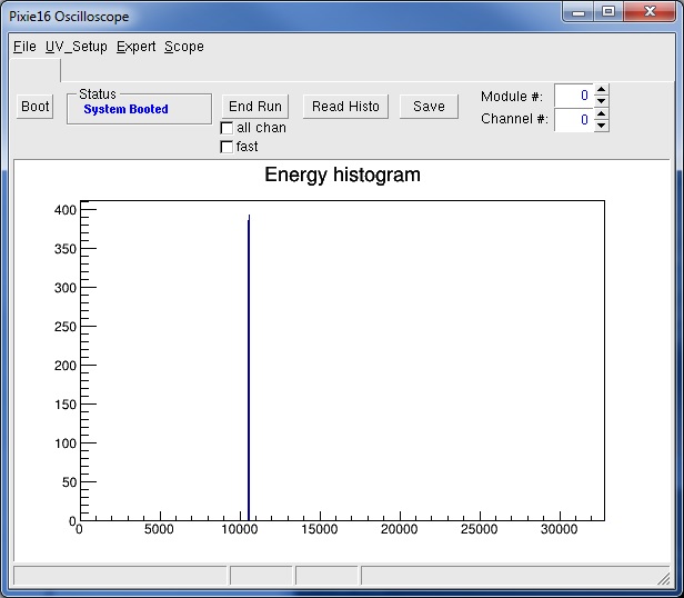
Stop data taking by clicking the End Run button. Normally you need to repeat the process described above for each channel you are using.
When running a multi-crate system, it is important to set a few more bits. Open up the CSRB dialog by going to Expert->ModCsrb. It is very important that all modules in the system have the MC checkbutton selected. Furthermore, the MAS and PUL checkbuttons should be checked for the module in slot 2 only.
Once all channels are set up, save the settings using the UV_Setup->Save2File menu command. In the file selection dialog that pops up, choose the .set file you specified in your cfgPixie16.txt file. This file will be loaded into the modules automatically when they are booted.
To configure Pixie-16 modules in a separate crate, you will have to exit nscope and start it again from the correct directory and computer. It is a good idea to set the parameters for each channel while attached to the hardware itself.
With all of the modules in the system configured using nscope and their settings files saved, you can now begin running the system with Readout. Unlike the single crate system, this is not as easily accomplished at the command line. The reason is that you need to open up multiple terminals on different hosts to tell each individual crate to start taking data. Remember the crates are connected at the hardware level, so unless you have all crates running, no triggers will be processed. The easiest way to run all crates together is to use the ReadoutGUI. We will describe how to do that in the next section.
There is nothing special about setting up the ReadoutGUI that pertains to the DDAS. The reader can learn all about how to register Readout programs to the ReadoutGUI in the standard NSCLDAQ documentation website. Because this document aims to be self contained, I will describe the process in detail here for our two crates.
The Readout programs for DDAS are going to be launched by the ReadoutGUI as ssh pipes. For that reason, it is paramount that the user can login to their own account without being prompted for a password. To accomplish this, follow the instructions at the portal help page.
It should be easy to determine whether this has been set up properly by typing:
ssh localhost
If properly set up, no password should have been requested. If you were prompted for a password, then something is amiss. Go back over the directions and make sure you followed them all exactly. If you are still being prompted for a password, contact someone that can help with this sort of issue. At the NSCL, you're best solution is to email helpme@nscl.msu.edu and providing a very detailed description of the behavior and a copy of all the error messages you received.
The "stagearea" is a hierarchy of directories with well-defined structure that ReadoutGUI uses to store data files. Typically, the toplevel directory of this is named stagearea. Because large volumes of data will be stored in this directory and only 2 GB are made available on the home directory of a standard experimental account, this directory should not actually live in the user's home directory. The canonical and recommended way of setting this up is to create a symbolic link in the user's home directory that points to the actual directory to be used for storage. For example, if an experimental account is named e12003, the actual directory for storage to be used is /events/e12003. Create a symbolic link to it in the home directory by typing
% ln -s /events/e12003 $HOME/stagearea
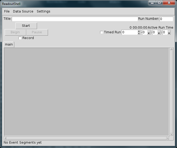
To launch the ReadoutGUI, the user should execute the following command:
$DAQROOT/ReadoutShell
At this point, one of three things should have happened.
The ReadoutGUI is not associated with any Readout programs by default and needs to be provided the information concerning the ones that will form the system.
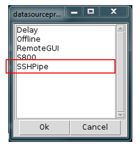
Select Data Source > Add... to add your first data provider. The data provider dialogue will prompt you to choose the type of data provider you are going to use. Select SSHPipe and then press the "Ok" button.
The data provider dialogue will prompt you to enter information for your first data source. Enter the path to your Readout program and any command line options that go with it. Press the "Ok" button.
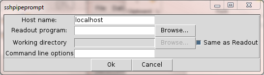
For crate 1, I have entered in the following information:
| Description | Value |
|---|---|
| Host name : | spdaq22 |
| Readout program | /usr/opt/ddas/VERSION/bin/DDASReadout |
| Working directory | /user/0400x/readout/crate_1 |
| Same as readout | Make sure it is unchecked |
| Command line options | --ring crate_1 --sourceid 1 |
VERSION should be the version of the ddas that is being used and should be something along the lines of 1.0-001.
There are a couple important things that need to be pointed out here. First is that the host name is the name of the computer that is physically attached to the PXI crate. The second aspect of these values warranting attention are the command line options. The first option, --ring, tells the DDASReadout program to output data to the ringbuffer on spdaq22 called crate_1. If the ringbuffer does not exist, it is created. Other components of the system can access its data by attaching to the ringbuffer tcp://spdaq22/crate_1. The other command line option, --sourceid, specifies the source id that will be assigned to the data from this readout program. If the user does not explicitly this parameter, the source id will default to 0.
To add crate 2 to the system, we simply repeat the same procedure. For my system, I used the following options:
| Description | Value |
|---|---|
| Host name : | spdaq05 |
| Readout program | /usr/opt/ddas/VERSION/bin/DDASReadout |
| Working directory | /user/0400x/readout/crate_2 |
| Same as readout | Make sure it is unchecked |
| Command line options | --ring crate_2 --sourceid 2 |
Once you have added both of the readout programs to the ReadoutGUI, you should be able to view that they have been added correctly. To do so, go to Data Source > List.
When the ReadoutGUI is exited, these settings are written to a configuration file that is loaded the next time ReadoutGUI is started.
To best understand the following tutorial steps, some basic idea of how the event builder is constructed is useful to have. The event builder is a process that accepts data from an arbitrary number of client processes. Internally it stores data labeled with different source ids in separate queues. Each client process is responsible for consuming data items from a ring buffer, ensuring each has the appropriate information for processing, and then passing the products (i.e. fragments) to the event builder for processing. At startup, the event builder has no clients. For that reason, we have to register the clients to it. The following sections will instruct the reader on how to enable the event builder itself and then also how to set up and register clients.
The event builder add-on to the ReadoutGUI is enabled by adding some TCL commands to the ReadoutCallouts.tcl script. Until now, this script has not been mentioned. It is just a standard TCL script that is sourced once when ReadoutGUI is launched. It must exist in one of three locations:
To enable the use of the event builder, cut and paste the following code into your ReadoutCallouts.tcl script.
package require evbcallouts

::EVBC::useEventBuilder

proc OnStart {} {
  ::EVBC::initialize -restart true -glombuild true -glomdt 100 -destring evb_out
}
The OnStart proc will be executed when the "Start" button is pressed. The ::EVBC::initialize proc will initialize the event builder with a few specific configuration options. Those options specify that the event builder will restart on each new run (-restart), event correlation will be enabled (-glombuild), events within 100 time units of each other will be correlated (-glomdt) and output in a single physics event, and the output will be put into the ring named built on localhost. The DDAS Readout program converts all timestamps into units of nanoseconds, so the -glomdt value will cause events within 100 ns to be correlated into a single built event.
The clients of the event builder are responsible for ensuring that the data items passed to them contain appropriate information for event building. These pieces of data are the source id, timestamp, and barrier type. The DDAS Readout program already adds these pieces of information to the data by means of the body header, so the client doesn't need to do anything more than access the existing information. The standard event builder client that is provided by NSCLDAQ, ringFragmentSource, has an option called --expectbodyheaders that causes it to use this preexisting information. We will be sure to specify this later.
For each stream of data that will be fed to the event builder, there must be an event builder client registered for it. Clients are added to the event builder using the EVBC::registerRingSource proc, which follow the EVBC::useEventBuilder call. For each of the data sources, add lines that had the following form:
::EVBC::registerRingSource sourceURI tstampLib id info expectBodyHeaders oneshotMode timeout
The ::EVBC::registerRingSource proc adds information about a client to a client manager. When the user begins a run, the manager will use the information provided to launch as many ringFragmentSource clients as have been registered.
Recall that the timestamp and source id are already defined by DDASReadout. For this reason, we do not need to provide a timestamp extraction function to the client by means of the tstampLib argument. It does require a placeholder, however, so we must pass an empty string, i.e. {}. The id argument must be provided and it must match the source id of the data in that stream. For my two crates, I will add the following two lines:
::EVBC::registerRingSource tcp://spdaq22/crate_1 {} 1 "Crate 1" 1 1 20
::EVBC::registerRingSOurce tcp://spdaq05/crate_2 {} 2 "Crate 2" 1 1 20
The empty string passed as a tstampLib argument is allowed by the client only because we told the client to expect that all of the information needed by the event builder is present in a body header (i.e. expectBodyHeaders = 1 or true). The ids were entered to match the values we passed each of the Readout programs in the command line options. It is VERY important that these match or else things will break. The info argument will be used as a label for the client in the event builder window. The second to last argument states that the client should exit on its own after a run is completed. The final argument specifies that all clients should exit if they do not observe the run end within 20 seconds of the time the first client observes it.
At this point, the event builder is enabled and the next press of the "Start" button will append a bunch of TCL widgets to the bottom of the ReadoutGUI.
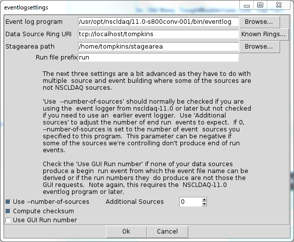
At some point, it will be necessary to save data to disk. ReadoutGUI has some reasonable defaults, but you should double check that the data recording is configured appropriately before beginning your first recorded data run. To do so, press the drop down menu button in Settings > Event Recording... The most common parameter in the dialog that will need to be changed is the "Data Source Ring URI". In our situation, we want to record the event built data that is outputted by the event builder. The name of this ring we declared above in the EVBC::initialize command to be evb_out. In that case, the value of the "Data Source Ring URL" should be tcp://localhost/evb_out. Be sure that the "stagearea path" has the correct path to the stagearea you created, the "Use \--number-of-sources" is checked and additional sources is set to 0. Finally, ensure the "Compute checksum" button is selected and the "Use GUI Run number" is NOT selected.
At this point, pressing the "Start" button will start the Readout programs in the system. It does NOT cause the Readout programs to commence data taking. After you press start, you should see a bunch of widgets added to the bottom of the ReadoutGUI window to control the event builder. These are for controlling the event builder. DDAS can take a long time to start up. You will have to wait for it to complete its initialization prior to pressing any more buttons. You will know that it has completed when the it outputs something like:
04/08/2016 15:46:29 : output : SSHPipe@spdaq22:1: Synch Wait OK 0

04/08/2016 15:46:29 : output : SSHPipe@spdaq22:1: In Synch OK 0

04/08/2016 15:46:29 : output : SSHPipe@spdaq22:1: Construct end command

04/08/2016 15:46:29 : output : SSHPipe@spdaq22:1: setup scalers for 2 modules

04/08/2016 15:46:29 : output : SSHPipe@spdaq22:1: Scalers know crate ID = 1

04/08/2016 15:46:29 : output : SSHPipe@spdaq22:1: Scalers know crate ID = 1
Once you have seen similar output for both the Readout programs, the system is ready to begin a run. The "Begin" button, which enables after the start transition is successful, will cause the data taking to begin. To end the run, simply press the "End" run button.
We are now going to inspect the data that is outputted from the event builder. To do so, attach the NSCLDAQ dumper program to the built ring. Assuming that you are logged onto the same machine that is running the event builder, you can do so with the following command:
$DAQBIN/dumper --source=tcp://localhost/evb_out --count=20
This should show you a stream of 20 data items printed to the terminal. Each physics event will have the following form:
Event 76 bytes long
Body Header:
Timestamp:    631110
SourceID:     0
Barrier Type: 0
004c 0000 a146 0009 0000 0000 0002 0000
0034 0000 0000 0000 0034 0000 001e 0000
0014 0000 a146 0009 0000 0000 0002 0000
0000 0000 000c 0000 0064 0c0c 4120 0008
f687 0000 0000 147f 08be 0000
The data in the built event is really just a bunch of fragments laid out contiguously in memory. A fragment has the following structure
| Top level | Data Type | Length(bytes) |
|---|---|---|
| Fragment header | timestamp | 8 |
| source id | 4 | |
| payload size | 4 | |
| barrier type | 4 | |
| Fragment payload | payload | <payload size> |
Furthermore, the payload is going to be structured as a ring item. Ring items, as you can read about in the NSCLDAQ documentation, consist of a header followed by a body with optional body header. In our case, the body will always have a body header because of the way DDAS Readout is designed. The layout of the physics event ring item (from DDAS) has the following form:
| Top level | Data type | Length (bytes) |
|---|---|---|
| Header | size | 4 |
| type | 4 | |
| Body Header | size | 4 |
| timestamp | 8 | |
| source id | 4 | |
| barrier type | 4 | |
| Body | Inclusive 16-bit word count | 4 |
| Data | ... | ... |
So let's back up to the dump of the built ring item that was provided above. It is composed of one or more fragments. When we parse the body, we will make use of the first 4 bytes of the body are an inclusive byte count of the entire body and the payload size to determine how many fragments there are and also when we have finished parsing the data. We can then look at the contents of the fragments to understand the event data. To illustrate this, the above raw data event will be decomposed into its pieces. The raw data dump is broken up into 16-bit words. To make it more easy to understand I will consolidate the chunks that go together and then label them.
| Dumped data | Translated data | Meaning |
|---|---|---|
| 004c 0000 | 0x0000004c | Inclusive size of built body |
| a146 0009 0000 0000 | 0x000000000009a146 | Frag #0 Header : timestamp |
| 0002 0000 | 0x00000002 | Frag #0 Header : source id |
| 0034 0000 | 0x00000034 | Frag #0 Header : payload size |
| 0000 0000 | 0x00000000 | Frag #0 Header : barrier type |
| 0034 0000 | 0x00000034 | Frag #0 Payload : ring item size |
| 001e 0000 | 0x0000001e | Frag #0 Payload : ring item type |
| 0014 0000 | 0x00000014 | Frag #0 Payload : body header size |
| a146 0009 0000 0000 | 0x000000000009a146 | Frag #0 Payload : body header timestamp |
| 0002 0000 | 0x00000002 | Frag #0 Payload : body header source id |
| 0000 0000 | 0x00000000 | Frag #0 Payload : body header barrier type |
| 000c 0000 | 0x0000000c | Frag #0 Payload : incl. 16-bit word count of body |
| 0064 0c0c | 0x0c0c0064 | Frag #0 Payload : Description of Pixie-16 module |
| 4120 0008 | 0x00084120 | Frag #0 Payload : 1st 32-bit word from Pixie-16 module |
| f687 0000 | 0x0000f687 | Frag #0 Payload : 2nd 32-bit word from Pixie-16 module |
| 0000 147f | 0x147f0000 | Frag #0 Payload : 3rd 32-bit word from Pixie-16 module |
| 08be 0000 | 0x000008be | Frag #0 Payload : 4th 32-bit word from Pixie-16 module |
Note that the body of this built event contains just a single piece of data from a Pixie-16 module. More specifically, it contains the data for a single channel read on that module. If we were seeing correlations between events, then we would have seen a whole bunch of data associated with a second fragment. We provide some simple tools to parse the structure of this built body so that you should never need to write your own parser. However, it is useful to have a general understanding of the structure for debugging purposes.
Let's dive a bit deeper into this rabbit hole by analyzing the data in the body of phyics events emitted from the DDAS Readout. I am referring to the last six rows of the above table. The first 32-bit word is an inclusive 16-bit word count in the body. It defines the extent of valid data for the event. The next 32-bit word contains hardware information that identifies the type of module that was read out. It has the following form:
| Bit range | Description |
|---|---|
| 00 : 15 | Sampling frequency (MSPS) |
| 16 : 23 | ADC resolution (# of bits) |
| 24 : 31 | Module revision |
Based on this knowledge we can determine that the module that produced this event is a revision 12, 12-bit, 100 MSPS digitizer. That is good, because I know the hardware in the crate I am reading out matches this description.
The remaining four 32-bit words are what the module emitted. The structure depends on the configuration of the device and you can read all about it in more detail in the Pixie-16 manual. We will only restrict ourselves to understanding the current configuration, which is to simply compute an energy. The structure of the data packet read from the module for a single event has the following form:
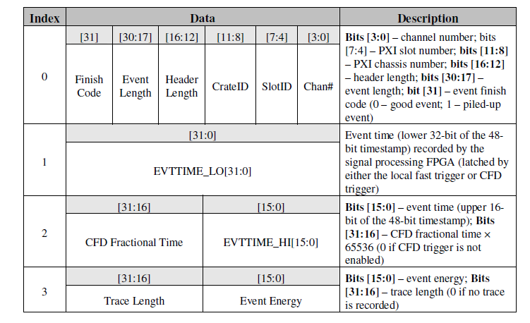
Based on this diagram, the first word, 0x00084120, tells us that the data corresponds to channel 0 of the module in slot 2 of crate 1. The header will be four 32-bit words long, the event is eight 16-bit words long, and that there was no pile-up detected. The second and third words, 0x0000f687 and 0x147f0000, are used to compute the raw timestamp of the event. The lower 32-bits of the timestamp come from the first of these and the upper 16-bits come from the lower 16-bits of the second. So the raw 48-bit timestamp is 0x00000000f687, which is 63111 in decimal. The 100 MSPS digitizers timestamp at 100 MHz, so a single clock tick is 10 ns, and DDAS Readout will convert a timestamp to nanoseconds. You can then see where the timestamp of 0x09a146 (i.e. 61110 in decimal) came from. The upper 16-bits of the second piece of data is a CFD time. These 16-bits are only present when we select CFD triggering. They provide a sub-clock correction to the timestamp we just computed. DDAS will compute this correction for you if you use the ddaschannel object provided by libddaschannel.so. The final 32-bit word, 0x000008be, tells us that the energy was 2238 and that the trace length is 0. This is all very reasonable.
Note that if you were to look at the data upstream of the event builder, the fragment header would be completely missing and you would only be seeing the payload. This is because the process of sending data through the event builder adds the fragment headers and builds the built event structure.
SpecTcl is the lab-supported framework for analyzing data online. The DDAS comes with some tools to use in unpacking DDAS data within the context of SpecTcl, DAQ::DDAS::DDASUnpacker and DAQ::DDAS::DDASBuiltUnpacker. These both provide support for parsing the raw data of DDAS for you. It is in your best interest to leverage these tools rather than writing your own parser. To learn how to use the DAQ::DDAS::DDASBuiltUnpacker in your SpecTcl, please refer to Analyzing DDAS Data in SpecTcl Tutorial.
 1.8.8
1.8.8

