8.4. How to set up the ScalerDisplay
Setting up the ScalerDisplay amounts to writing a basic configuration file and then specifying to the program where the scaler data is to be read from.
The configuration file is a simple TCL script that associates names with channels and defines how the data is to be displayed. Though the script is to be written in the TCL programming language, it is written at a very high level. In fact, you should be able to put one together without any knowledge of the language by following our examples. At the same time, the user who knows TCL can write standard TCL code within their script and it will be interpreted as expected.
In the following examples, we will develop a complete configuration script suitable for the ScalerDisplay as well as describe how to launch the program. The first example will treat an experiment that consists of a single source of scaler data and the second example will build on the resulting configuration file of the first example to demonstrate how to deal with multiple sources of scaler data.
8.4.1. Single Readout Experiment Example
Here are some assumptions that we will make for our first example:
A Readout program already exists that periodically reads 16 channels of scaler data, but only the first 5 channels are meaningful and worthy of displaying.
The Readout program is going to be running on the local machine (i.e. localhost) and is outputting its data to the ring named "output".
Given these assumptions, we have only two steps to take. The first is to generate a configuration script. Start by creating an empty file called scaler.def.
spdaqXX> touch scaler.def
The ScalerDisplay starts up with zero knowledge of the scaler channels it will display as well as how it is to organize those channels. Our first step is to inform the program which scaler data it should be concerned with. We do so by associating names to our scaler channels using the channel command. It takes as its arguments the name and the channel identifier. The channel identifier is composed of two mandatory arguments: a channel index and a source id. The channel identifier has the format "ch.id" where "ch" is the channel index and "id" is the source id. If you are unsure of the source id, you can inspect the data with the dumper program. [1] Let's assume that we know the source id was 1. We would then have to add the following five lines to our configuration file.
channel raw_10hz_clock 0.1
channel live_10hz_clock 1.1
channel raw_trigger 2.1
channel live_trigger 3.1
channel labr_cfd 4.1
Note that if you determined that your scaler data has no source id (i.e. no body header), then you should identify the channel by only its index. In that case, we would have written:
channel raw_10hz_clock 0
channel live_10hz_clock 1
channel raw_trigger 2
channel live_trigger 3
channel labr_cfd 4
That is all you really need to register scaler channels to the
ScalerDisplay. However, you can also provide options to the channel
command. Three of these are worth mentioning. The first option,
-incremental, specifies whether the data is incremental
or not via a boolean value. An incremental scaler is one in which the
counters are cleared after every read. In this way, each read provides
an incremental change to the scaler since the last read and clear. A
nonincremental scaler is when no clear follows the read. Each read value
provides the accumulated value in that case. By default, channels are
assumed to be incremental. Let's assume that our channels were
nonincremental, as a result we will rewrite each of our lines as
follows:
channel -incremental 0 raw_10hz_clock 0.1
channel -incremental 0 live_10hz_clock 1.1
channel -incremental 0 raw_trigger 2.1
channel -incremental 0 live_trigger 3.1
channel -incremental 0 labr_cfd 4.1
The two other options that are worth mentioning are the
-lowlim and -hilim options, because
they set up visual alarms for when the rate of a channel is outside of
what is expected to be normal. Let's set those parameters for our
live_10hz_clock to exemplify their usage. We want to make sure we are
always more than 70% live, which means we should never have a rate on
our live_10hz_clock channel that is less than 7. We also want to make
sure that it never goes over 10, because that would not make sense for a
10 Hz clock. We can set visual alarms for this scenario by rewriting the
line for the live_10hz_clock channel as this:
channel -lowlim 7 -hilim 10 live_10hz_clock 1.1
Now that we have these limits set, the corresponding information for the live_10hz_clock will be highlighted in green if the rate drops below 7, it will highlight in red if it goes above, and it will be displayed as any other channel (black text on white background) if it is between 7 and 10. There is a checkbutton clearly visible on the ScalerDisplay that will allow you to enable and disable the alarms. The alarms for any of the other channels can be set up in like manner.
At this point the ScalerDisplay will know the scaler data by its associated name and we can begin defining how to display it. Part of our assumptions was that the remaining 11 channels of data in our data stream were not meaningful to display. Because we did provide lines in our scaler.def file to define these, they will simply be ignored. Our first step towards displaying the data is to add a page to display the channels on. We will create a blank page named "scalers" whose title is "Scalers" by writing:
page scalers Scalers
You can register an arbitrary number of pages and they show up as tabs on the ScalerDisplay.
The next step is to add scaler channels to the page we just created. We will do so with the display_single command to do that. Its arguments are the page name and then the channel name. Each subsequent call will add a row to the page below the last. Here is what we need to add to display our scaler channels on the "scalers" page.
display_single scalers raw_10hz_clock
display_single scalers live_10hz_clock
display_single scalers raw_trigger
display_single scalers live_trigger
display_single scalers labr_cfd
At this point, the configuration script could be considered complete because it would display the numbers for the five scaler channels we described. However, let's add some more pieces to it for the sake of show and tell. We could also have the ScalerDisplay display the ratio of the first two channels as a measure of the system live time. We do that with the display_ratio command. It takes the page name as its first argument, the name of the channel for the numerator as the second argument, and then the name of the channel for the denominator as the last. To clearly separate the displayed ratio from the single channel data, I am going to add a blank row in between them. This can be done using the blank command; it takes the page name as an argument. So here we add the ratio of the raw_10hz_clock to live_10hz_clock to the "scalers" page after a blank line.
blank scalers
display_ratio scalers raw_10hz_clock live_10hz_clock
Ok. Now we have our complete configuration file.
To launch the ScalerDisplay, we first need to define an environment variable called SCALER_RING. It contains a list of the ring buffers where the scaler data is to be read from. In our case that would be "tcp://localhost/output" because our ring buffer is named "output" and it lives on "localhost". You would do so by typing the following at the command line:
spdaqXX> export SCALER_RING="tcp://localhost/output"
The next step is to launch the ScalerDisplay program with the configuration script as an argument. In our case, we would type the following:
spdaqXX> $DAQBIN/ScalerDisplay scaler.def
You should see the following window pop up.
![]()
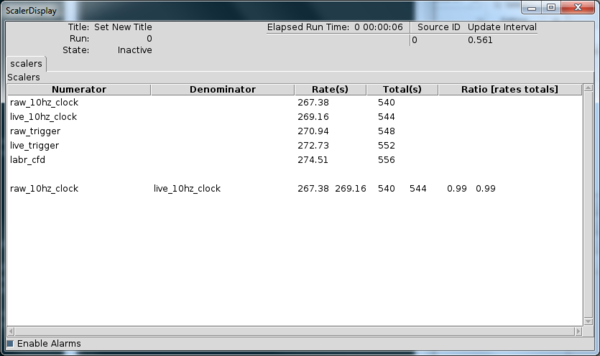
When the scaler data arrives into the ring buffer that was specified in SCALER_RING, the ScalerDisplay will show valid data. It will look something like this:
8.4.2. Two Readout Program Example
Now we will describe how to set up the ScalerDisplay to manage scaler data that was contributed by more than 1 readout program. For brevity, let's assume that one of the Readout programs was the same as the previous example. For this reason, our scaler.def we created in the last example is still valid and we will just add on to it. The second readout program we will consider will introduce data that has been labeled as source id 2 and we will only care about channels 2-4 of this source. So, let's start by adding a second page to our scaler display using the page command. Add this to your scaler.def file:
page id2 Source2
We now have a second page that will contain all of our scaler data from source id 2. Next we will associate names with our channels
channel hpge_cfd0 2.2
channel hpge_cfd1 3.2
channel scint_cfd0 4.2
Notice how all of the channel identifiers ended with a ".2" to indicate that they are labeled source id 2. Alright and then we will add our channels to be displayed on the page we created called Source2.
display_single id2 hpge_cfd0
display_single id2 hpge_cfd1
display_single id2 scint_cfd0
Done. Now let's make things more interesting. The ScalerDisplay provides a strip chart for monitoring the trends of the scaler values. You can register channels to be plotted on the strip chart using the stripparam and stripratio commands. The stripparam takes a single argument, the channel name, and the stripratio command takes two commands, the channel name of the numerator followed by the denominator. We will plot register the trend of the labr_cfd by itself as well as the ratio of our live time clocks. To do so, we add the following to our scaler.def file:
stripparam labr_cfd
stripratio live_10hz_clock raw_10hz_clock
stripconfig timeaxis 1200
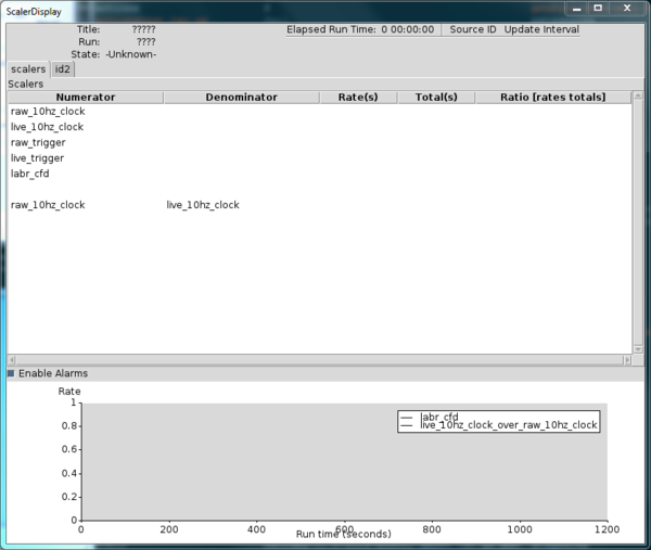
The last line that called the stripconfig command specified that the past 1200 seconds of history would be displayed by the stripchart. When we launch the ScalerDisplay the next time, it will have two tabs that allow switching between the scaler value of each source and will also have a strip chart at the bottom of it.
Now we are done editing our configuration script. We next just need to change our SCALER_RING environment variable. In most cases when we have multiple Readout programs, the event builder will be used to merge together the two data streams. The result will be that all of our scaler data will be available to read from a single ring buffer downstream of the event builder. In this case, we simple need to list the name of that single ring buffer. Let's assume we called it "built" and it lives on spdaqX. We would write:
spdaqXX> export SCALER_RING="tcp://spdaqX/build"
We would then launch the ScalerDisplay in the same way we did the last example.
Consider though the case that we did not want to monitor the scaler data downstream of the event builder. Maybe instead we cared to monitor it when it lived in two separate rings. One could imagine doing this for diagnostic purposes. Whatever the reasons that would inspire someone to do this, let's show how it is done. Of course, this is just done by redefining our SCALER_RING environment variable. The SCALER_RING environment variable is interpreted as a list of ring names so we just need to list them. Let's assume we have the scaler data for source id 0 in the ring buffer named "output" on localhost. We will then assume that the source id 2 data is in the ring named "output2" on localhost. We can then set the environment variable to:
spdaqXX> export SCALER_RING="tcp://localhost/output tcp://localhost/output2"
The ScalerDisplay then launches as normal taking the path to the configuration file as its argument. With the addition of the strip chart you will see a slightly different looking window pop up than in the previous example:
8.4.3. Run Summary Output of ScalerDisplay
Besides just providing a convenient display of the scaler data in an experiment, the program will also generate summary files of complete runs. It produces three output files
Summary of scaler information as formatted text (runnnnn.report file)
Summary of scaler information formatted as a csv (runnnnn.csv)
Postscript file of the strip chart (runnnnn-stripchart.ps)
The summary files of the scaler information contains all of the known scaler channel data displayed as a table. It lists the total, average, and standard deviation for each scaler channel. A sample output of the .report file might look like this:
Run     :  0
Title   :  Set New Title
Started :  Thu Mar 05 13:42:08 EST 2015
Ended   :  Thu Mar 05 13:42:43 EST 2015
Elapsed : 0 00:00:34

+---------------+-----+------------+------------+
|Name           |Total|Average Rate|Rate std-dev|
+---------------+-----+------------+------------+
|hpge_cfd0      |0    |0.00        |0.00        |
|hpge_cfd1      |0    |0.00        |0.00        |
|labr_cfd       |184  |5.28        |2.70        |
|live_10hz_clock|181  |5.20        |2.66        |
|live_trigger   |183  |5.26        |2.68        |
|raw_10hz_clock |180  |5.17        |2.66        |
|raw_trigger    |182  |5.23        |2.67        |
|scint_cfd0     |0    |0.00        |0.00        |
+---------------+-----+------------+------------+
And the corresponding .csv file will look something like this:
0,Set New Title,Thu Mar 05 13:42:08 EST 2015,Thu Mar 05 13:42:43 EST 2015,34
hpge_cfd0,0,0.0,0.0
hpge_cfd1,0,0.0,0.0
labr_cfd,184,5.284622896203114,2.6973414456885623
live_10hz_clock,181,5.198460566373715,2.6600670279318797
live_trigger,183,5.255902119593314,2.6797992677490887
raw_10hz_clock,180,5.1697397897639155,2.65799093865138
raw_trigger,182,5.227181342983514,2.6673506246677756
scint_cfd0,0,0.0,0.0
The .csv file does not explicitly label the content of each column as the .report file does. One can understand the columns in the first row to be in the following order:
Run number
Title string
Date and time at which the run started
Date and time at which the run ended
Total length of run in seconds
The second and subsequent lines contain information in the following order from left to right:
Name of the scaler channel
Total number of counts in that channel during duration of run
Average count rate in channel for duration of run
Standard deviation of the count rate over duration of run
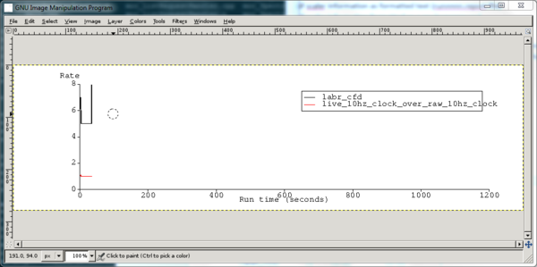
The .ps file can be opened in your favorite postscript viewer. I opened it in gimp for lack of a better option:
spdaqXX> gimp run0000-stripchart.ps
After working through the gimp import dialog, I see this: